An Overview of Statistical Learning:
- Statistical learning refers to the set of tools for modeling and understanding of complex datasets.
- Alternative Definition: Statistical learning refers to a vast set of tools for understanding data.
- These tools can be classified as supervised or unsupervised.
- Supervised statistical learning involves building a statistical model for predicting, or estimating, an output based on one of more inputs.
- With unsupervised statistical learning, there are inputs but no supervising output.
- These tools can be classified as supervised or unsupervised.
- Alternative Definition: Statistical learning refers to a vast set of tools for understanding data.
- Regression problem: predicting a continuous or qualitative output value.
- Classification problem: predicting a non-numerical value (categorical or qualitative output).
- Clustering problem: Situations in which we only observe input variables, with no corresponding output. In clustering problems we are not trying to predict an output variable.
A Brief History of Statistical Learning:
- At the beginning of the nineteenth century, Legendre and Gauss published papers on the method of least squares, which implemented the earliest form of what is now known as linear regression.
- Linear regression is used to predict quantitative values.
- In 1936, Fisher proposed linear discriminant analysis to predict qualitative values.
- In the 1940's, various authors put forth an alternative approach called logistic regression.
- In the early 1970's, Nelder and Wedderburn coined the term generalized linear models for an entire class of statistical learning methods that include both linear and logistic regression as special cases.
- Not until the 1980's were non-linear methods feasible due to lack of computational power.
- This is when classification and regression trees were introduced.
- In 1986, Hastie and Tibshirani coined the term generalized additive models for a class of non-linear extensions to generalized linear models.
Notation and Simple Matrix Algebra:
- We will use n to represent the number of distinct data points, or observations, in our sample.
- We will use p to denote the number of variables that are available for use in making predictions.
- We will let x
ijrepresent the value of the j^th^ variable for the i^th^ observation, where i = 1,2,...,n and j = 1, 2,..., p. - i will be used to index the samples or observations (from 1 to n) and j will be used to index the variables (from 1 to p).
- We will let X denote a n x p matrix whose (i, j)th element is x
ij. - Vectors are by default represented as columns.
- The ^T^ notation denotes the transpose of a matrix or vector.
- We use y
ito denote the i^th^ observation of the variable on which we wish to make predictions.
Linear vs. Non-Linear Models:
- Linear methods often have advantages over their non-linear competitors in terms of interpretability and sometimes also accuracy.
Supervised Learning
- Outcome measurement Y (also called dependent variable, response, target)
- Vector of p predictor measurements X (also called inputs, regressors, covariates, features, independent variables)
- We have training data (x
1, y1),...,(xN, yN). These are observations (examples, instances) of these measurements.
Regression vs. Classification (Supervised Learning):
- In the regression problem, Y is quantitative (e.g. price, blood pressure)
- In the classification problem, Y takes values in a finite unordered set (survived/died, digit 0-9, cancer class of tissue sample)
- The objective of both regression and classification is to, on the basis of the training data we would like to:
- Accurately predict unseen test cases.
- Understand which inputs affect the outcome, and how.
- Assess the quality of our predictions and inference.
Unsupervised Learning:
- No outcome variable, just a set of predictors (features) measured on a set of samples.
- Objective is more fuzzy - find groups of samples that behave similarly, find features that behave similarly, find linear combinations of features with the most variation.
- Difficult to know how well you are doing.
- Different from supervised learning, but can be useful as a pre-processing step for supervised learning.
Statistical Learning versus Machine Learning:
- Machine learning arose as a subfield of Artificial Intelligence.
- Statistical learning arose as a subfield of Statistics
- There is much overlap - both fields focus on supervised and unsupervised problems:
- Machine learning has a greater emphasis on large scale applications and prediction accuracy.
- Statistical learning emphasized models and their interpretability, and precision and uncertainty.
- But the distinction has become more and more blurred, and there is a great deal of 'cross-fertilization.'
Notation:
- Response or Target variable is normally referred to as Y
- Feature, or Input, or Predictor variables are referred to as X
- A model is written as Y = f(X) + Error
- Error is a catch all to capture measurement errors and other discrepancies.
- Error is the irreducible error.
Intoduction:
- Input variables go by different names; predictors, independent, features, or sometimes just variables
- The output variable is often called the response variable or dependent variable.
- The relationship between target variable (Y) and feature (X) can be written in the very general from: Y = f(X) + Error
- Here f is some fixed but unknown function for X
1,.....Xpand Error is a random error term, which is independent of X and has mean zero. - In this formulation, f represents the systematic information that X provides about Y.
- It is important to note that the irreducible error term will always have a mean of zero.
- In essence, statistical learning refers to a set of approaches for estimating f.
- Here f is some fixed but unknown function for X
Why Estimate f:
- There are two main reasons that we may wish to estimate f:
- Prediction
- In many situations, a set of inputs X are readily available. but the output Y cannot be easily obtained. In this setting, since the error term averages to zero, we can predict Y using Y-hat = f-hat(X), where f-hat represents the resulting prediction for Y.
- The accuracy of Y-hat as a prediction for Y depends on two quantities, which we will call the reproducible error and the irreducible error.
- The focus of this textbook is on techniques for estimating f with the aim of minimizing the reducible error.
- Inference
- We want to understand the relationship between X and Y, or more specifically, to understand how Y changes as a function of X
1,...,X2. - Answer the questions:
- Which predictors are associated with the response?
- What is the relationship between the response and each predictor?
- Can the relationship between Y and each predictor be adequately summarized using a linear equation, or is the relationship more complicated?
- We want to understand the relationship between X and Y, or more specifically, to understand how Y changes as a function of X
- Prediction
How Do we Estimate f?:
- We will always assume we have observed a set of n different data points.
- These observations are called the training data because we will use these observations to train, or teach, our method how to estimate f.
- Out goal is to apply a statistical learning method to the training data in order to estimate the unknown function f.
- Most statistical learning methods for this task can be characterized as either:
- Parametric
- Involve a two-step model-based approach. First, make an assumption about the functional form, or shape of f (i.e. linear). Second, use a procedure that uses the training data to fit or train the model (i.e. Ordinary Least Squares).
- Parametric means reducing the problem of estimating f down to one of estimating a set of parameters.
- Non-parametric
- Do not make explicit assumptions about the functional form of f. Instead they seek an estimate of f that gets as close to the data points as possible without being too rough or wiggly.
- More data is needed to fit non-parametric models.
- Parametric
- Overfitting: the model follows the errors, or noise, too closely.
The Trade-Off Between Prediction Accuracy and Model Interpretability:

- If we are mainly interested in inference, then restrictive models are much more interpretable.
- If you are more interested in prediction, then flexible models are much more predictive.
Supervised Versus Unsupervised Learning:
- Most statistical learning problems fall into one of two categories:
- Supervised Learning
- For each observation of the predictor measurement(s) x there is an associated response measurement y.
- We wish to fit a model that relates the response to the predictors, with the aim of accurately predicting the response for future observations (predictions) or better understanding the relationship between the response and the predictors (inference).
- Examples: Linear and logistic regression
- Unsupervised Learning
- For every observation we observe a vector of measurements x, but no associated response y.
- Referred to as unsupervised because we lack a response variable that can supervise our analysis.
- We seek to understand the relationship between the variables or between the observations.
- Example: Clustering (to ascertain whether the observations fall into relatively distinct groups).
- Supervised Learning
Regression Versus Classification Problems:
- Variables can be characterized as either quantitative or qualitative (also known as categorical).
- Quantitative variables take on numerical values.
- Example: Age, height, income
- Qualitative variables take on values in one of K different classes or categories.
- Example: Sex, cancer diagnosis
- We tend to refer to problems with a quantitative response as regression problems, while those involving a qualitative response are often referred to as classification problems.
- We tend to select statistical learning methods on the basis of whether the response is quantitative or qualitative.
Assessing Model Accuracy:
- There is no free lunch in statistics: no one method dominates all others over all possible data sets.
Measuring the Quality of Fit:
- In order to evaluate the performance of a statistical learning method on a given data set, we need some way to measure how well its predictions actually match the observed data.
- In the regression setting, the most commonly-used measure is the mean squared error (MSE).
- The MSE will be small if the predicted responses are very close to the true responses, and will be large if for some of the observations, the predicted and true responses differ substantially.
- We want to choose the method that gives the lowest test MSE, as opposed to the lowest training MSE.
- As model flexibility increases, training MSE will decrease, but the test MSE may not.
- When a given method yields a small training MSE but a large test MSE, we are said to be overfitting the data.
- When we overfit the training data, the test MSE will be very large because the supposed patterns that the method found in the training data simply don't exist in the test data.
- Note that regardless of whether or not overfitting has occurred, we almost always expect the training MSE to be smaller than the test MSE because most statistical learning methods either directly or indirectly seek to minimize the training MSE.
- Overfitting refers specifically to the case in which a less flexible model would have yielded a smaller test MSE.
- One important method is cross-validation, which is a method for estimating the test MSE using the training data.
- The degrees of freedom is a quantity that summarizes the flexibility of a curve.
- A more restricted and hence smoother curve has fewer degrees of freedom than a wiggly curve.
The Bias-Variance Trade-Off:
- Variance refers to the amount by which f-hat would change if we estimated it using a different training data set.
- Ideally, the estimate for f should not vary too much between training sets.
- In general, more flexible statistical methods have higher variance.
- Bias refers to the error that is introduced by approximating a real-life problem, which may be extremely complicated, by a much simpler mode.
- Generally, more flexible methods result in less bias.
- Ideally, we want to select a statistical learning method that simultaneously achieves low variance and low bias.
- In reality, a general rule is, as we use more flexible methods, the variance will increase and the bias will decrease.
- Good test set performance of a statistical learning method requires low variance as well as low squared bias.
- This is referred to as a trade-off because it is easy to obtain a method with extremely low bias but high variance (for instance, by drawing a curve that passes through every single training observation) or a method with very low variance but high bias (by fitting a horizontal line to the data).
- The challenge lies in finding a method for which both the variance and the squared bias are low.
- This is referred to as a trade-off because it is easy to obtain a method with extremely low bias but high variance (for instance, by drawing a curve that passes through every single training observation) or a method with very low variance but high bias (by fitting a horizontal line to the data).
The Classification Setting:
- When the target variable is qualitative instead of quantitative, the most common approach to quantifying the accuracy of our estimate f-hat is the training error rate, the proportion of mistakes that are made if we apply our estimate f-hat to the training observations.
- A good classifier is one for which the test error is smallest.
K-Nearest Neighbors:
- The choice of K has a drastic effect on the KNN classifier obtained.
- When K=1, the decision boundary is overly flexible and finds patterns in the data that don't correspond to the Bayes decision boundary.
- This corresponds to a classifier that has low bias, but very high variance.
- As K grows, the method becomes less flexible and produces a decision boundary that is close to linear.
- This corresponds to a low-variance but high-bias classifier.
- When K=1, the decision boundary is overly flexible and finds patterns in the data that don't correspond to the Bayes decision boundary.
- As in the regression setting, the training error rate consistently declines as the flexibility increases.
- In both the regression and classification settings, choosing the correct level of flexibility is critical to the success of any statistical learning method.
Chapter 2 Exercises:
- For each of parts (a) through (d), indicate whether we would generally expect the performance of a flexible statistical learning method to be better or worse than an inflexible method.
a) The sample size n is extremely large, and the number of predictors p is small.
- Answer: Better, a more flexible approach will fit the data closer and with the large sample size a better fit than an inflexible approach would be obtained. b) The number of predictors p is extremely large, and the number of observations n is small.
- Answer: Worse, a flexible method would overfit the small number of observations. c) The relationship between the predictors and response is highly non-linear.
- Answer: Better, with more degrees of freedom, a flexible model would obtain a better fit. d) The variance of the error terms is extremely high.
- Answer: Worse, flexible methods fit to the noise in the error terms and increase variance.
- Explain whether each scenario is a classification or regression problem, and indicate whether we are most interested in inference or prediction. Finally, provide n and p. a) We collect a set of data on the top 500 firms in the US. For each firm we record profit, number of employees, industry, and the CEO salary. We are interested in understanding which factors affect CEO salary. * Answer: Regression. Inference. n = 500 firms in the US and p = profit, number of employees, and industry. b) We are considering launching a new product and wish to know whether it will be a success or failure. We collect data on 20 similar products that were previously launched. For each product, we have recorded whether it is a success or failure, price charged for the product, marketing budget, competition price, and ten other variables. * Answer: Classification. Prediction. n = 20 similar products and p = price charged for the product, marketing budget, competition price, and ten other variables. c) We are interested in predicting the % chance in the US dollar in relation to the weekly changes in the world stock markets. Hence, we collect weekly data for all of 2012. For each week we record the % change in the dollar, the % change in the US market, the % change in the British market, and the % change in the German market. * Answer: Regression. Prediction. n = weekly data for all of 2012 and p = the % change in the US market, the % change int he British market, and the % change in the German market.
- Sketch bias, variance, training error, test error, and Bayes (or irreducible error curves, on a single plot, as we go from less flexible statistical learning methods towards more flexible approaches).
- Answer: Sketch Here
Explain why each of the five curves displayed in the sketch.
- Bias: Decreases monotonically because increases in flexibility yield a closer fit
- Variance: Increases monotonically because increases in flexibility yield overfitting
- Training Error: Decreases monotonically because increases in flexibility yield a closer fit
- Test Error: Concave because increase in flexibility yields a closer fit.
- Bayes (irreducible) error: defines the lower limit for the test error. When the training error is lower than the irreducible error, overfitting has taken place.
4a) Describe a real-life application in which classification might be useful. Describe the response, as well as the predictors. Is the goal of the application inference or prediction?
- Answer: To predict whether a patient has cancer. The response variable would be a positive or negative diagnosis for cancer. The predictors may be age, medical history, and weight. The goal is prediction.
4b) Describe a real-life application in which regression might be useful. Describe the response, as well as the predictors. Is the goal of the application inference or prediction?
- Answer: A team win prediction model. The response would be wins. The predictors may be previous season record, strength of schedule, and coach. This goal would be prediction.
4c) Describe a real-life application in which cluster analysis might be useful?
- Answer: Player position archetype clustering.
- What are the advantages and disadvantages of very flexible (versus a less flexible) approach for regression or classification? Under what circumstances might a more flexible approach be preferred to a less flexible approach? When might a less flexible approach be preferred?
- Answer: The advantage for a very flexible approach for regression or classification are obtaining a better fit for non-linear models, thus decreasing bias. The disadvantages for a very flexible approach for regression or classification are the requirement to estimate a greater number of parameters, following the noise too closely (overfitting), and increasing variance.
- Answer: A more flexible approach would be preferred to a less flexible approach when we are interested in prediction and not in interpretability of the results. A less flexible approach would be preferred to a more flexible approach when we are interested in inference and the interpretability of the results.
- Describe the difference between a parametric and a non-parametric statistical learning approach. What are the advantages of a parametric approach to regression or classification (as opposed to a non-parametric approach)? What are its disadvantages?
- Answer: A parametric approach reduces the problem of estimating f down to one of estimating a set of parameters because it assumes a form for f. A non-parametric approach does not assume a functional form for f and so requires a very large number of observations to accurately estimate f.
- Answer: The advantages of a parametric approach to regression or classification are the simplifying of modeling f to a few parameters and not as many observations are required compared to a non-parametric approach. The disadvantages of a parametric approach to regression or classification are a potential to inaccurately estimate f if the form of f assumed is wrong or to overfit the observations if more flexible models are used.
KNN Example:
- Nearest neighbor models can be pretty good for small p (predictors) i.e., p <= 4 and large-ish N (observations).
- Nearest neighbor methods can be lousy when p is large because of the curse of dimensionality.
- Nearest neighbors tend to be far away in high dimensions.
Parametric and Structured Models:
- Parametric models don't suffer from the curse of dimensionality in most cases since they are not very flexible.
- The linear model is an important example of a parametric model.
- Although it is almost never correct, a linear model often serves as a good and interpretable approximation to the unknown true function f(X).
Some trade-offs:
- Prediction accuracy versus interpretability
- Linear models are easy to interpret; thin-plate splines are not.
- Good fit versus over-fit or under-fit
- Parsimony versus black-box
- We often prefer a simpler model involving fewer variables over a black-box predictor involving them all.
Bias-Variance Trade-Off:
- Typically as the flexibility of f-hat increases, its variance increases, and its bias decreases. So choosing the flexibility based on average test error (MSE) amounts to a bias-variance trade-off.
Introduction:
- Linear regression is a useful supervised learning tool for predicting a quantitative response.
- Many of the most advanced statistical learning approaches can be seen as generalizations or extensions of linear regression.
Simple Linear Regression:
- Straightforward approach for predicting a quantitative response Y on the basis of a single predictor variable X.
- Assumes there there is approximately a linear relationship between X and Y.
- Sometimes described by saying that we are regression Y on X.
- Equation: Y=B
0+ B1X- B
0and B1are two unknown constants that represent the intercept and slope terms in the linear model. - Together B
0and B1are known as the model coefficients or parameters.
- B
Estimating the Coefficients:
- We want to find an intercept B
0and slope B1such that the resulting line is as close as possible to the data points.- There are a number of ways of measuring closeness. However, by far the most common approach involves minimizing the least squares criterion.
- The least squares approach chooses B
0and B1to minimize the Residual Sum of Squares.
Assessing the Accuracy of the Coefficient Estimates:
- The true relationship between X and Y takes the form Y = f(X) + error for some unknown function f, where error is a mean-zero random error term.
- This the linear function can be written: Y = B
0+ B1X + error - The error term is a catch-all for what we miss with this simple model: the true relationship is probably not linear, there may be other variables that cause variation in Y, and there may be measurement error.
- This the linear function can be written: Y = B
- An unbiased estimator does not systematically over- or underestimate the true parameter.
- We interpret the p-value as follows: a small p-value indicates that it is unlikely to observe such a substantial association between the predictor and the response due to chance.
- If we see a small p-value, then we can infer that there is an association between the predictor and the response.
Assessing the Accuracy of the Model:
- The quality of a linear regression fit is typically assessed using two related quantities: the residual standard error (RSE) and the R^2^ statistic.
Residual Standard Error:
- Roughly speaking, RSE is the average amount that the response will deviate from the true regression line.
- The RSE is considered a measure of the lack of fit of the model to the data.
- RSE is an absolute measure of lack of fit of the model to the data, meaning it is measured in the units of the target variable Y and that it's not always clear what constitutes a good RSE.
R^2^ Statistic:
- Provides an alternative measure of fit, which takes the form of a proportion, the proportion of variance explained.
- Always takes on a value between 0 and 1
- Independent of the scale of Y
- Equation: 1 - (RSS/TSS)
- R^2^ measures the proportion of variability in Y that can be explained by X.
- An R^2^ statistic that is close to 1 indicates that a large proportion of the variability in the response has been explained by the regression.
- A number near 0 indicates that the regression did not explain much of the variability in the response; this might occur because the linear model is wrong, or the inherent error is high, or both.
- The R^2^ statistic is a measure of the linear relationship between X and Y.
Multiple Linear Regression:
- We interpret the coefficient of each predictor as the average effect on Y of a one unit increase in X
j, holding all other predictors fixed. - Parameters in multiple linear regression are estimated using the same least squares approach as simple linear regression with the goal of minimizing the sum of squared residuals.
- Various statistics can be used to judge the quality of a model including Mallow's C
p, Akaike Information Criterion (AIC), Bayesian Information Criteria (BIC), and adjusted R^2^. - There are three classical approaches to variable selection:
- Forward Selection
- Sequentially add variables one at a time starting with the null model.
- Can always be used.
- A greedy approach that might include variables early that later become redundant. (Mixed selection can remedy this).
- Backward Selection
- Start with all variables in the model and remove the variable with the largest p-value in sequential order.
- Cannot be used if p > n.
- Mixed Selection
- Combination of forward and backward selection.
- Forward Selection
- Two of the most common numerical measures of model fit are the RSE and R^2^, the fraction of variance explained.
- R^2^ will always increase when more variables are added to the model, even if those variables are only weakly associated with the response.
- In terms of qualitative predictors, also called factors, there will always be one fewer dummy variable than the number of levels.
- The level with no dummy variable is known as the baseline.
Extensions of the Linear Model:
- The standard linear regression model makes two highly restrictive assumptions that are often violated in practice:
- The relationship between the predictors and response are additive, meaning that the effect of changes in a predictor X on the response Y is independent of the values of the other predictors.
- The predictors and response are linear, meaning that the change in the response Y due to a one-unit change in X is constant, regardless of the value X.
- Some common classical approaches for extending the linear model and relaxing these two assumptions:
- One way of extending this model to allow for interaction effects is to include a third predictor, called an interaction term, which is constructed by computing the product of multiple predictors.
- The hierarchical principle states that if we include an interaction in a model, we should also include the main effects, even if the p-values associated with their coefficients are not significant.
- A very simple ways to directly extend the linear model to accommodate non-linear relationships is to use polynomial regression.
- A simple approach for incorporating non-linear associations in a linear model is to include transformed versions of the predictors in the model.
- The approach for extending the linear models to accommodate non-linear relationships is known as polynomial regression.
- One way of extending this model to allow for interaction effects is to include a third predictor, called an interaction term, which is constructed by computing the product of multiple predictors.
Potential Problems of Linear Regression:
- Non-linearity of the response-predictor relationship
- The linear regression model assumes that there is a straight-line relationship between the predictors and the response.
- If the true relationship isn't linear, then virtually all of the conclusions that we draw from the fit are suspect.
- Residual plots are a useful graphical tool to identify non-linearity.
- Ideally, the residual plot will show no discernible pattern.
- The presence of a pattern may indicate a problem with some aspect of the linear model.
- If the residual plot indicates that there are non-linear associations in the data, then a simple approach is to use non-linear transformations of the predictors, such as log(X), sqrt(X), and X^2^
- Correlation of error terms
- An important assumption of the linear regression model is that the error terms are uncorrelated.
- If the error terms are correlated, we may have an unwarranted sense of confidence in our model.
- Non-constant variance of error terms
- An assumption of the linear regression model is that the error terms have a constant variance.
- One can identify non-constant variances in the errors, or heteroscedasticity, from the presence of the funnel shape in the residual plot.
- When faced with the problem, one possible solution is to transform the response Y using a concave function such as log(Y) or sqrt(Y)
- Such a transformation results in a greater amount of shrinkage of the larger responses, leading to a reduction in heteroscedasticity.
- Outliers
- An outlier is a point for which the predicted value is far from the value predicted by the model.
- Residual plots can be used to identify outliers.
- However, it can be difficult to decide how large a residual needs to be before we consider the point to be an outlier.
- To overcome this, instead of plotting the residuals, plot the studentized residuals, computed by dividing each residual by its estimated standard error. Observations whose studentized residuals are greater than 3 in absolute value are possible outliers.
- High-leverage points
- While outliers are observations for which the response y is unusual given the predictor x, high leverage points have an unusual value for x.
- In order to quantify an observation's leverage, we compute the leverage statistic.
- The leverage statistic is always between 1/n and 1.
- If a given observation has a leverage statistic that greatly exceeds (p+1)/n, then we may suspect that the corresponding point has high leverage.
- Collinearity
- Refers to the situation in which two or more predictor variables are closely related to one another.
- Since two or more predictors tend to increase or decrease together, it can be difficult to determine how each one separately is associated with the response.
- Collinearity reduces the accuracy of the estimates of the regression coefficients.
- The power, or probability of detecting a non-zero coefficient, is reduced by collinearity.
- A simple way to detect collinearity is to look at the correlation matrix of the predictors.
- Unfortunately, not all collinearity problems can be detected by inspection of the correlation matrix: it is possible for collinearity to exist between three or more variables even if no pair of variables has a particularly high correlation. We call this situation multicollinearity has a particularly high correlation matrix.
- A better way to assess multicollinearity is to compute the variance inflation factor (VIF).
- The smallest possible value of VIF is 1, which indicates the complete absence of collinearity.
- A rule of thumb is that a VIF value that exceeds 5 or 10 indicates a problematic amount of collinearity.
- When faced with the problem of collinearity, there are two simple solutions. The first is to drop one of the problematic variables from the regression. The second solution is to combine the collinear variables together into a single predictor.
Comparison of Linear Regression with K-Nearest Neighbors:
- Linear regression is an example of parametric approach because it assumes a linear functional form for f(X).
- Advantage of Parametric Models: Easier to fit because one need estimate only a small number of coefficients.
- Disadvantage of Parametric Models: They make strong assumptions about the form of f(X).
- If the specified functional form is far from the truth and prediction accuracy is our goal, then the parametric method will perform poorly.
- KNN is one of the simplest and best-known non-parametric methods.
- The parametric approach will outperform the non-parametric approach if the parametric form that has been selected is close to the true for of f.
- As a general rule, parametric methods will tend to outperform non-parametric approaches when there is a small number of observations per predictor.
Chapter 3 Exercises: 2) Explain the difference between the KNN classifier and the KNN regression methods. * Answer: The final result of KNN classifier is the classification output for Y (qualitative), where was the output for the KNN regression predicts the quantitative value for Y.
- Linear regression is a simple approach to supervised learning.
- It assumes that the dependence of Y on X
1, X2,...Xpis linear.- True regression functions are never linear!
- Although it may seem overly simplistic, linear regression is extremely useful both conceptually and practically.
- Assumes a model Y = B
0+ B1X + error where B0and B1are two unknown constants that represent the intercept and slope, also known as coefficients or parameters and an error term.- If the slope is 0, then there is no relationship between Y and X
- Residual: difference between a predicted value and the actual value.
- The standard error of an estimator reflects how it varies under repeated sampling.
- These standard errors can be used to compute confidence intervals. A 95% confidence interval is defined as a range of values such that with 95% probability, the range will contain the true unknown value of the parameter.
- Standard errors can also be used to perform a hypothesis tests on the coefficients. The most common hypothesis test involves testing the null hypothesis of:
- H
O: There is no relationship between X and Y versus the alternative hypothesis. - H
A: There is some relationship between X and Y
- H
- We use statistical software to compute the p-value to complete the hypothesis test.
- In multiple linear regression, we interpret each coefficient as the average effect on Y of a one unit increase in X holding all other predictors fixed.
- The ideal scenario is when the predictors are uncorrelated
- Then coefficients can be estimated and tested separately.
- Correlations amongst predictors cause problems
- The variance of the coefficients tends to increase, sometimes dramatically
- Interpretations become hazardous.
Model Selection:
- To determine if at least on predictor is useful we examine the F-statistic.
- The larger the F-statistic, the most evidence that one or more predictors is useful in the model.
- How to decide on the important variables:
- The most direct approach is called all subsets or best subsets regression: we compute the least squares fit for all possible subsets and then choose between them based on some criterion that balances training error with model size.
- However, we often can't examine all possible models, since their are 2^p^ of them; for example when p = 40 there are over a billion potential models.
- Instead we need an automated approach that searches through a subset of the predictors.
- Two options of doing so are:
- Forward Selection
- Begin with the null model - a model that contains an intercept but no predictors.
- Fit p simple linear regressions and add to the null model the variable that results in the lowest RSS.
- Add to that model the variable that results in the lowest RSS amongst all two-variable models.
- Continue until some stopping rule is satisfied; for example when all remaining variables have a p-value above some threshold.
- Backward Selection
- Start with all variables in the model
- Remove the variable with the largest p-value - that is, the variable that is the least statistically significant.
- The new (p - 1)-variable model is fit, and the variable with the largest p-value is removed.
- Continue until a stopping rule is reached. For instance, we may stop when all remaining variables have a significant p-value defined by some significance threshold.
- Forward Selection
- To determine the effectiveness of a model, we could use any of the following metrics:
- Mallow's C~p~
- Akaike Information Criterion (AIC)
- Bayesian Information Criterion (BIC)
- Adjusted R^2^
- Cross-Validation
Qualitative Predictors:
- Some predictors are not quantitative but are qualitative, taking a discrete set of values.
- These are called categorical predictors or factor variables
- To handle categorical predictors we use dummy variables.
- There will always be one fewer dummy variable than the number of categories. The level with no dummy variable is known as the baseline.
- Removing the additive assumption: interactions and nonlinearity
- The hierarchy principle: If we include an interaction in the model, we should also include the main effects, even if the p-values associated with their coefficients are not significant.
- The rationale for this principle is that interactions are hard to interpret in a model without main effects - their meaning is changed.
- Generalizations of the Linear Model
- Classification problems: logistic regression, support vector machines
- Non-linearity: kernel smoothing, splines and generalized additive models, nearest neighbor methods
- Interactions: Tree-based methods, bagging, random forests and boosting (these also capture non-linearities)
- Regularized fitting: ridge and lasso regression
Introduction:
- In classification the target variable is qualitative instead of quantitative.
- Often qualitative variables are referred to as categorical.
- Predicting a qualitative response for an observation can be referred to as classifying that observation, since it involves assigning the observation to a category or class.
- In reality, classification is really predicting the probability that the observation is part of each category of a qualitative variable, as the basis for making the classification.
- In this sense, classification behaves very similarly to regression.
- Three of the most common classifiers are logistic regression, linear discriminant analysis, and K-Nearest Neighbors
Why Not Linear Regression?
- In general, there is no natural way to convert a qualitative response that is ready for linear regression.
Logistic Regression:
- Logistic regression models the probability that Y belongs to a particular category.
- In logistic regression, we use the logistic function.
- To fit the model we use a method called maximum likelihood.
- Maximum likelihood is a very general approach that is used to fit many of the non-linear models.
- In the regression setting, the least squares approach is in fact a special case of maximum likelihood.
- In logistic regression, increasing predictor variable X by one unit changes the log odds of target variable Y by the coefficient of X.
Linear Discriminant Analysis:
- Linear discriminant analysis is popular when we have more than two response classes.
- Why do we need another method, when we have logistic regression?
- When the classes are well-separated, the parameter estimates for the logistic regression model are surprisingly unstable. Linear discriminant analysis does not suffer from this problem.
- If n is small and the distribution of the predictors X is approximately normal in each of the classes, the linear discriminant model is again most stable than the logistic regression model.
- The higher the ratio of parameters p to number of samples n, the most we might expect overfitting to play a role.
- The overall performance of a classifier, summarized over all possible thresholds, is given by the area under the ROC curve (AUC).
Quadratic Discriminant Analysis:
- QDA serves as a comparison between the non-parametric KNN and linear LDA and logistic regression approaches.
- Assumes a quadratic decision boundary.
- Can accurately model a wider range of problems than can the linear methods.
- Though not as flexible as KNN, QDA can perform better in the presence of a limited number of training observations because it does make some assumptions about the form of the decision boundary.
A Comparison of Classification Method:
- Though their motivations differ, the logistic regression and LDA methods are closely connected.
- They each produce a linear decision boundary.
- They each are parametric.
- Although, they differ in their fitting procedures.
- KNN is different in that it is non-parametric, no assumptions are made about the shape of the decision boundary.
- Thus, we can expect KNN to dominate LDA and logistic regression when the decision boundary is highly non-linear.
- KNN does not tell us which predictors are important since there are no coefficients similar to LDA and logistic regression.
- No one method will dominate the others in every situation.
- When the true decision boundaries are linear, then the LDA and logistic regression approaches will tend to perform well.
- When the boundaries are moderately non-linear Quadratic Discriminant Analysis may give better results.
- For much more complicated decision boundaries, a non-parametric approach such as KNN can be superior.
- e = 2.71828 is a mathematical constant (Euler's nubmer)
- In logistic regression we use maximum likelihood to estimate the parameters.
- This likelihood gives the probability of the observed zeros and ones in the data.
- We select the parameters to maximize the likelihood of the observed data.
- Logistic regression ensures that our estimate for p(X) lies between 0 and 1.
- We generally don't care about the p-value of the intercept.
- In logistic regression with more than two classes, we fit a linear function for each class.
- Really, only K - 1 linear functions are needed as in 2-class logistic regression.
- Multiclass logistic regression is also referred to as multinomial regression.
- The approach of discriminant analysis is to model the distribution of X in each of the classes separately, and then use Bayes theorem to flip things around and obtain Pr(Y|X)
- When we use normal (Gaussian) distribution for each class, this leads to linear or quadratic discriminant analysis.
- Other distributions can be used as well.
- Why discriminant analysis over logistic regression?
- When the classes are well-separated, the parameter estimates for the logistic regression model are surprisingly unstable. Linear discriminant analysis does not suffer from this problem.
- If n is small and the distribution of the predictors X is approximately normal in each of the classes the linear discriminant model is again more stable than the logistic regression model.
- Linear discriminant analysis is popular when we have more than two response classes, because it also provides low-dimensional views of the data.
- Bayes decision boundaries, yield the fewest misclassification errors, among all possible classifiers. (i.e., the true decision boundaries)
- In practice, these are unknown.
- Logistic Regression vs. LDA
- Logistic regression is discriminative learning
- LDA is generative learning.
- In practice, the results of each are often very similar.
- Provides a non-linear discriminant boundary between classes.
- Logistic regression can also fit quadratic boundaries like QDA, by explicitly including quadratic terms in the model.
- Naive Bayes
- Assumes features are independent in each class.
- Useful when p is large, and so multivariate methods like QDA and LDA break down.
- Despite strong assumptions, naive bayes often produces good classification results.
- Summary:
- Logistic regression is very popular for classification, especially when K = 2.
- LDA is useful when n is small, or the classes are well separated, and Gaussian assumptions are reasonable. Also, when K > 2.
- Naive Bayes is useful when p is very large.
Introductions:
- Resampling methods involve repeatedly drawing samples from a training set and refitting a model of interest on each sample in order to obtain additional information about the fitted model.
- Two of the most commonly used resampling methods are:
- Cross validation
- Used to estimate the test error associated with a given statistical learning method in order to evaluate its performance, or to select the appropriate level of flexibility.
- The process of evaluating a model's performance is known as model assessment, whereas the process of selecting the proper level of flexibility for a model is known as model selection.
- Bootstrapping
- Used in several contexts, most commonly to provide a measure of accuracy of a parameter estimate or of a given statistical learning method.
- Cross validation
Cross-Validation:
- The test error is the average error that results from using a statistical learning method to predict the response on a new observation - that is, a measurement that was not used in training the method.
- In the absence of a test set, we can estimate the test error rate by holding out a subset of the training observations from the fitting process and then applying the statistical learning method to those held out observations.
The Validation Set Approach:
- Involves randomly dividing the available set of observations into two parts, a training set and a validation set or holdout set.
- The model is fit on the training set, and the fitted model is used to predict the responses for the validation set.
- The resulting validation set error rate provides an estimate for the test error rate.
- The validation set approach has two drawbacks:
- The validation estimate of the test error rate can be highly variable, depending on precisely which observations are included in the training set and which observations are included in the validation set.
- Since statistical methods tend to perform worse when trained on fewer observations, this suggests that the validation set error rate may tend to overestimate the test error rate for the model fit on the entire data set.
- The cross validation method is a refinement of the validation set that addresses these two issues.
Leave-One-Out Cross-Validation:
- Similar to validation set approach but instead of splitting the data in half, it fits the model on n - 1 observations (training data) and uses 1 observation as the validation data.
- This leads to an unbiased estimate for the test error.
- However, it is a poor estimate because it is highly variable, since it is based on a single observation.
- Also, can be computationally expensive since you have to fit the model multiple times on n - 1 observations.
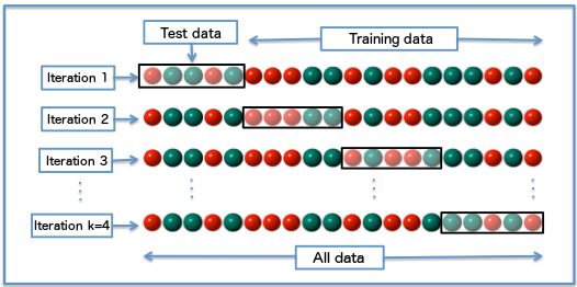
k-Fold Cross-Validation:
- Involves randomly dividing the set of observations into k groups, or folds, of approximately equal sizes.
- The first fold is treated as the validation set and the model is fit on the remaining k - 1 folds.
- This procedure is repeated k times, with each time a different fold serving as the validation set.
- This process results in k estimates of the test error, which we average to get the final estimate of the test error.
- Leave-One-Out Cross-Validation (LOOCV) is a special case of k-fold cross validation in which k is set to equal n.
- In practice, one typically performs k-fold CV using k=5 or k=10.
- When we perform cross-validation, our goal is to determine how well a given statistical learning procedure can be expected to perform on independent data.
Bias-Variance Trade-Off for k-Fold Cross-Validation:
- K-fold CV with k < n has a computational advantage to LOOCV.
- It also gives more accurate estimates of the test error rate due to the bias-variance trade-off.
- There is a bias-variance trade-off associated with the choice of k in k-fold cross-validation. Typically, given these considerations, one performs k-fold cross validation using k=5 or k=10 as these values have been shown empirically to yield error rate estimates that suffer neither from excessively high bias nor from very high variance.
The Bootstrap:
- Used to quantify the uncertainty associated with a given estimator or statistical learning method.
- Allows us to use a computer to emulate the process of obtaining new sample sets, so that we can estimate the variability of an estimator without generating additional samples.
- Rather than repeatedly obtaining independent data sets from the population, we instead obtain distinct data sets by repeatedly sampling observations from the original data set.
- Sampling is done with replacement, which means that the same observations can occur more than once in the bootstrap data set.
- Two resampling methods: cross-validation and the bootstrap
- These methods refit a model of interest to samples formed from the training set, in order to obtain additional information about the fitted model.
- For example, they provide estimates of test-set prediction error, and the standard deviation and bias of our parameter estimates.
- Recall the distinction between test error and the training error:
- The test error is the average error that results from using a statistical learning method to predict the response on a new observation, one that was not used in training the method.
- In contrast, the training error can be easily calculated by applying the statistical learning method to the observations used in its training.
- But the training error rate often is quite different from the test error rate, and in particular the former can dramatically underestimate the latter.
- The more complex a model, the lower the training error in most cases.
- In most cases where we don't have a large designated test set, we either:
- Make mathematical adjustments to the training error rate in order to estimate the test error rate.
- these include the C
pStatistic, AIC, and BIC.
- these include the C
- Estimate the test error by holding out a subset of the training observations from the fitting process, and then applying the statistical learning method to those held out of observations.
- Make mathematical adjustments to the training error rate in order to estimate the test error rate.
- Validation-Set Approach:
- Randomly divide the available set of samples into two parts: a training set and a validation or holdout set.
- The model is fit on the training set, and the fitted model is used to predict the response for the observations in the validation set.
- The resulting validation-set error provides an estimate of the test error. This is typically assessed using MSE in the case of a quantitative response and misclassification rate in the case of a qualitative (discrete) response.
- Drawbacks of validation-set approach:
- The validation estimate of the test error can be highly variable, depending on precisely which observations are included in the training set and which observations are included in the validation set.
- In the validation approach, only a subset of the observations - those that are included in the training set rather than in the validation set - are used to fit the model.
- This suggests that the validation set error may tend to overestimate the test error for the model fit on the entire data set.
- Because, the more data we have to fit a model, the lower the error.

- Widely used approach for estimating test error.
- Estimates can be used to select best model, and to give an idea of the test error of the final chosen model.
- Idea is to randomly divide the data into K equal-sized parts. We leave our part k, fit the model to the other K-1 parts (combined), and then obtain predictions for the left-out kth part.
- This is done in turn for each part k=1,2,...K, and then the results are combined.
- Leave One Out Cross Validation: The same process but the number of k is equal to the number of observations.
- Sometimes useful, but typically doesn't shake up the data enough.
- The estimates from each fold are highly correlated and hence the average can have high variance.
- K = 5 or 10 provides a good comparison for the bias-variance tradeoff.
- Wrong: Filtering out predictors before running cross-validation.
- Right: Filter our predictors during cross-validation (i.e., filter out certain predictors in each fold of the CV).
- The bootstrap is a flexible and powerful statistical tool that can be used to quantify the uncertainty associated with a given estimator or statistical learning method.
- For example, it can provide an estimate of the standard error of a coefficient, or a confidence interval for that coefficient.
- The bootstrap approach allows us to use a computer to mimic the process of obtaining new data sets, so that we can estimate the variability of our estimate without generating additional samples.
- Rather than repeatedly obtaining independent data sets from the population, we instead obtain distinct data sets by repeatedly sampling observations from the original data with replacement.
- Each of these 'bootstrap data sets' is created by sampling with replacement, and is the same size as our original dataset. As a result some observations may appear more than once in a given bootstrap data set and some not at all.
- In time series data, we must use blocks of consecutive observations and sample those with replacement since time series data is correlated.
- Primarily used to obtain standard errors of an estimate.
- Also, provides approximate confidence intervals for a population parameter
Introduction:
- The linear model has distinct advantages in terms of inference and, on real-world problems, is often surprisingly competitive in relation to non-linear methods.
- The simple linear model can be improved upon by replacing plain least squares fitting with some alternative fitting procedures.
- Alternative fitting procedures can yield better prediction accuracy and model interpretability.
- Prediction Accuracy: By constraining or shrinking the estimated coefficients, we can often substantially reduce the variance at the cost of a negligible increase in bias. This can lead to substantial improvements in the accuracy with which we can predict the response for observations not used in model training.
- Model Interpretability: By constraining or shrinking the estimated coefficients, sometimes to zero, we can obtain a model that is more easily interpreted.
- Least squares, in comparison, is unlikely to yield any coefficients that are exactly zero.
- Three common alternatives to using least squares:
- Subset Selection: This approach involves identifying a subset of the p predictors that we believe to be related to the response. We then fit a model using least squares on the reduced set of variables.
- Shrinkage: This approach involves fitting a model involving all p predictors. However, the estimated coefficients are shrunken towards zero relative to the least squares estimates.
- Also known as regularization.
- Has the effect of reducing variance.
- Dimension Reduction: Projecting the p predictors into a smaller dimensional subspace and then using those resulting predictors to fit a linear regression model by least squares.
Subset Selection:
-
Two main subset selection techniques:
- Best Subset Selection
- Fit a separate least squares regression for each possible combination of the p predictors.
- We then look at all of the resulting models, with the goal of identifying the one that is best.
- The number of possible models is equal to 2^p^
- While best subset selection is a simple and conceptually appealing approach, it suffers from computational limitations.
- Best subset selection becomes computationally infeasible for values of p greater than 40.
- Stepwise Selection Two kinds: 1) Forward Stepwise Selection * Considers a much smaller set of models as opposed to best subset selection. * Begins with a model containing no predictors, and then add predictors to the model, one-at-a-time, until all of the predictors are in the model. At each step the variable that gives the greatest additional improvement to the fit is added to the model. * Downside is unlike best subset selection, doesn't evaluate every possible model and thus might not select the optimal model. * Can be used when the number of predictors p is larger than the number of observations n. 2) Backward Stepwise Selection * Similar to forward stepwise selection, considers a much smaller set of models as opposed to best subset selection. * Begins with the full least squares model containing all p predictors, and then iteratively removes the least useful predictor, one-at-a-time. * Like forward step selection, doesn't see every possible model and thus, might not select the optimal model. * Requires that the number of observations n is larger than the number of predictors p. 3) Hybrid Approaches * Variables are added to the model sequentially, similar to forward selection, but after adding each new variable, the method can then remove variables that no longer provide an improvement in the model fit.
- The best subset, forward stepwise, and backward stepwise selection approaches generally give similar but not identical models.
Choosing the Optimal Model:
- The model containing all of the predictors will always have the smallest RSS and largest R^2^, since these quantities are related to the training error.
- However, training error can be a poor estimate of the test error.
- We instead want to select the model with the lowest test error.
- To estimate the test error we must either make adjustments to the training error to account for the bias due to overfitting or use cross-validation.
- Therefore, RSS and R^2^ are not suitable for selecting the best model among a collection of models with different numbers of predictors.
- Best Subset Selection
Cp, AIC, BIC, and Adjusted-R^2^:
- The training set training set MSE is generally an under-estimate of the test MSE.
- MSE = RSS/n
- The training error will decrease as more variables are included in the model, but the test error may not.
- Therefore, training set RSS and training set R^2^ cannot be used to select from among a set of models with different numbers of variables.
- However, we can adjust the training error to account for the bias added due to overfitting.
- The most common four adjustments are:
- Mallow's C
p(Smaller the better) - Akaike Information Criterion (AIC) (Smaller the better)
- Bayesian Information Criterion (BIC) (Smaller the better)
- Adjusted R^2^ (Larger the better)
- Unlike R^2^, Adjusted R^2^ pays a price for the inclusion of unnecessary variables in the model.
- Mallow's C
- The most common four adjustments are:
Cross Validation:
- Has an advantage to AIC, BIC, C
p, and Adjusted R^2^ in that it provides a direct estimate of the test error and makes fewer assumptions about the true underlying model. - Can be used in a wider range of model selection.
- Historically, cross-validation was not computationally feasible so statisticians relied on AIC, BIC, C
p, and Adjusted-R^2^. Nowadays, cross-validation is a better option.
Shrinkage Methods:
- As an alternative to fitting a linear model that contains a subset of predictors, we can fit a model containing all p predictors using a technique that constrains or regularizes the coefficient estimates, or equivalently, that shrinks the coefficients towards zero.
- By shrinking the coefficients we can significantly reduce their variance.
- The two best-known techniques for shrinking the regression coefficients towards zero are ridge regression and the lasso.
Ridge Regression:
- Uses a shrinking penalty,
$\lambda$ .- When
$\lambda$ = 0, the penalty term has no effect and ridge regression will produce the same estimates as least squares. - AS
$\lambda$ increases, the impact of the penalty term grows, and the ridge regression coefficient estimates approach zero. - The intercept never shrinks in ridge regression.
- When
- It is best to apply ridge regression after standardizing the predictors so that they are all on the same scale.
Why Does Ridge Regression Improve Over Least Squares:
- Least squares tends to have no bias, but high variance.
- Ridge regression significantly decreases variance with only a slight increase in bias.
- As
$\lambda$ increases, the flexibility of the ridge regression fit decreases, leading to decreased variance but increased bias.
- As
- In essence, ridge regression trades a small increase in bias for a large decrease in variance.
- Hence, ridge regression works best in situations where the least squares estimates have high variance.
- Ridge regression has substantial computational benefits over any of the subset selection methods.
- You only ever fit one ridge regression model compared to 2^p^ models needed to fit best subset selection.
The Lasso:
- The one downside of ridge regression, is it will include all p predictors in the final model.
- This may not be a problem for prediction accuracy, but it can create a challenge in model interpretation in settings in which the number of variables p is quite large.
- The lasso overcomes the problem by forcing coefficients to exactly zero.
- This is a form of natural variable selection.
- Because of this Lasso models are more easily interpretably than ridge models.
- Lasso uses an L1 penalty, while regression uses an L2 penalty.
- When
$\lambda$ = 0, then the lasso simply gives the least squares fit, and when$\lambda$ becomes sufficiently large, the lasso gives the null model in which all of the coefficient estimates equal zero.
Comparing the Lasso and Ridge Regression:
- The lasso has a major advantage over ridge regression in that it produces simpler and more interpretable models that involve only a subset of the predictors.
- However, in prediction accuracy neither ridge regression nor the lasso will universally dominate the other.
Dimension Reduction Methods:
- Dimension reduction methods transform the predictors and then fit a least squares model using the transformed variables.
- They take the p predictors and find a smaller number predictors M that are a linear combination of the original p predictors.
- Two most common dimension reduction methods:
- Principal Component Analysis
- Partial Least Squares
Principal Components Analysis:
- Approach for deriving a low-dimensional set of features from a large set of variables.
- The first principal component is the linear combination that yields the highest variance.
- The second principal component is perpendicular or orthogonal to the first principal component.
- In general, you can construct up to p principal components.
- Although, in practice you would not do this.
- You would then use these principal components in a least squares regression model.
- The idea is that often a small number of principal components suffice to explain most of the variability in the data.
- PCA in regression will tend to do well in cases in which the first few principal components are sufficient to capture most of the variation in the predictors as well as the relationship with the response.
- PCA is not a feature selection method as it's predictors are linear combinations of the original predictors.
- PCA regression is more closely related to ridge regression than Lasso.
- The number of principal components to use in the model is determined via cross-validation.
- Standardize all predictors before computing principal components.
Partial Least Squares:
- A supervised alternative to PCA regression.
- Similar process to PCA regression, but it uses the response variable in order to identify new features.
High-Dimensional Data:
- Most traditional statistical techniques for regression and classification are intended for the low-dimensional setting in which n, the number of observations, is much greater than p, the number of features.
- Over history, most problems have been low-dimensional problems with few predictors. Now with technological advances, most problems are high-dimensional with many predictors.
- Data sets containing more features than observations are often referred to as high-dimensional.
- Classical approaches such as least-squares regression are not appropriate for this setting.
- Because of the curse of dimensionality.
- Instead use ridge, lasso, and PCA regression.
- Regularization or shrinkage plays a key role in high-dimensional problems
- Despite its simplicity, the linear model has distinct advantages in terms of its interpretability and often shows good predictive performance.
- However, we can perform on linear models using alternatives to least squares.
- Why consider alternatives to least squares?
- Prediction accuracy: especially when p > n, to control the variance.
- Model Interpretability: By removing irrelevant features - that is, by setting the corresponding coefficient estimates to zero - we can obtain a model that is more easily interpreted.
- Three classes of feature selection:
- Subset selection: We identify a subset of the p predictors that we believe to be related to the response. We then fit a model using least squares on the reduced set of variables.
- Example: Best subset selection
- Shrinkage: We fit a model involving all p predictors, but the estimated coefficients are shrunken towards zero relative to the least squares estimates. This shrinkage (also known as regularization) has the effect of reducing variance and can also perform variable selection.
- Dimension Reduction: We project the p predictors into a M-dimensional subspace, where M < p. This is achieved by computing M different linear combinations, or projections, of the variables. Then these M projections are used as predictors to fit a linear regression model by least squares.
- Subset selection: We identify a subset of the p predictors that we believe to be related to the response. We then fit a model using least squares on the reduced set of variables.
- For computational reasons, best subset selection cannot be applied with very large p.
- A rule of thumb: if p is < 10 then it may be possible to create all possible models, but if p > 10 it is likely impractical.
- Best subset selection may also suffer from statistical problems when p is large: larger the search space, the higher the chance of finding models that look good on the training data, even though they might not have any predictive power on the future.
- Thus an enormous search space can lead to overfitting and high variance of the coefficient estimates.
- For both of these reasons, stepwise methods, which explore a far more restricted set of models, are attractive alternatives to best subset selection.
- Forward stepwise selection begins with a model containing no predictors (null model), and then adds predictors to the model one-at-a-time, until all of the predictors are in the model.
- In particular, at each step the variable that gives the greatest additional improvement to the fit is added to the model.
- We're looking at a smaller subset of all possible models.
- Computational advantage over best subset selection is clear.
- However, it is not guaranteed to find the best possible model out of all 2^p^ models containing subsets of the p predictors.
- Like forward stepwise selection, backward stepwise selection provides an efficient alternative to best subset selection.
- However, unlike forward stepwise selection, it begins with the full least squares model containing all p predictors (full model), and then iteratively removes the least useful predictor, one-at-a-time.
- Like forward stepwise selection, backward stepwise selection is not guaranteed to yield the best model containing a subset of the p predictors.
- Backward selection requires that the number of samples n is larger than the number of variables p (so that the full model can be fit).
- In contrast, forward stepwise can be used even when n < p, and so is the only viable subset method when p is very large.
- There are two approaches to estimating test error:
- We can indirectly estimate test error by making an adjustment to the training error to account for the bias do to overfitting
- We can directly estimate the test error, using either a validation set approach or a cross-validation approach as discussed in previous lectures.
- C
p, AIC, BIC, and Adjusted R^2^ are approaches to indirectly estimate test error by making an adjustment to the training error (approach #1 from above)- These techniques adjust the training error for the model size, and can be used to select among a set of models with different numbers of variables.
- Used to determine which models with different number of variables is best.
- If you have a good model these should all have similar results.
- BIC is more likely to give you a model with fewer features than AIC and Mallow's C
pas it penalizes more for additional features.
- Smaller values of AIC, BIC, and Mallow's C
pmeans a better model, while larger values of R^2^ means a better model. - AIC, BIC, and Mallow's C
pgeneralizes to other models, while R^2^ only works for linear regression.
- This procedure has an advantage relative to AIC, BIC, Mallow's C
pand Adjusted R^2^, in that is provides a direct estimate of the test error, and doesn't require an estimate of the error variance. - It can also be used in a wider range of model selection tasks, even in cases where it is hard to pinpoint the model degrees of freedom (e.g., the number of predictors in the model) or hard to estimate the error variance.
- One standard error rule: Choose the simplest model that comes within one standard error of the minimum error of all models.
- Two types of shrinkage methods: ridge regression and the lasso
- The subset selection methods use least squares to fit a linear model that contains a subset of the predictors.
- As an alternative, we can fit a model containing all p predictors using a technique that constrains or regularizes the coefficient estimates, or equivalently, that shrinks the coefficient estimates towards zero.
- Shrinking the coefficient estimates can significantly reduce their variance.
- Always standardize your feature matrix before applying ridge or lasso regression.
- Ridge is L2 penalty.
- Ridge regression does have one obvious disadvantage: unlike subset selection, which will generally select models that involve just a subset of the variables, ridge regression will include all p predictors in the final model.
- The Lasso is a relatively recent alternative to ridge regression that overcomes this disadvantage by forcing coefficients to zero.
- The Lasso is an L1 penalty.
- As with ridge regression, the lasso shrinks the coefficient estimates toward zero.
- However, in the case of the lasso, the L1 penalty has the effect of forcing some of the coefficient estimates to be exactly equal to zero when the tuning parameter
$\lambda$ is sufficiently large. - Hence, much like best subset selection, the lasso performs variable selection.
- We say that the lasso yields sparse models - that is, models that involve only a subset of the variables.
- As in ridge regression, selecting a good value of
$\lambda$ for the lasso is critical; cross-validation is again the method of choice. - Neither ridge regression nor the lasso will universally dominate the other.
- In general, one might expect the lasso to perform better when the response is a function of only a relatively small number of predictors.
- However, the number of predictors that is related to a response is never known a priori for real data sets.
- A technique such as cross-validation can be used in order to determine which approach is better on a particular data set.
- As for subset selection, for ridge regression and lasso we require a method to determine which of the models under consideration is best.
- That is, we require a method selecting a value for the tuning parameter
$\lambda$ or equivalently, the value of the constraint s.
- That is, we require a method selecting a value for the tuning parameter
- Cross-validation provides a simple way to tackle this problem.
- We choose a grid of
$\lambda$ values, and compute the cross-validation error rate for each value of$\lambda$ .
- We choose a grid of
- We then select the tuning parameter value for which the cross-validation error is smallest.
- Finally, the model is re-fit using all of the available observations and the selected value of the tuning parameter.
- Dimension reduction methods are a class of approaches that transform the predictors and then fit a least squares model using the transformed variables.
- Two-step procedure; find principal components and then fit them using a least-squares regression.
- The first principal component is that (normalized) linear combination of the variables with the largest variance.
- The second principal component has largest variance, subject to being uncorrelated with the first. And so on.
- Hence with many correlated original variables, we replace them with a small set of principal components that capture their joint variation.
- Determine the number of principal components by using a scree plot.
- Summary of Principal Component Regression:
- PCR identifies linear combinations, or directions, that best represent the predictors.
- These directions are identified in an unsupervised way, since the response Y is not used to help determine the principal component directions.
- That is, the response does not supervise the identification of the principal components.
- Consequently, PCR suffers from a potentially serious drawback: there is no guarantee that the directions that best explain the predictors will also be the best directions to use for predicting the response.
- Summary of Partial Least Squares:
- Like PCR, PLS is a dimension reduction method, which identifies linear combinations of original features and then fits a linear model via OLS using these M new features.
- But unlike PCR, PLS identifies these new features in a supervised way - that is, it makes use of the response Y in order to identify new features that not only approximate the old features well, but also that are related to the response.
- Roughly speaking, the PLS approach attempts to find directions that help explain both the response and the predictors.
- In practice, PLS does not give better results than PCR. PCR is more simple than PLS and thus is used more often.
Introduction:
- While standard linear regression have advantages over other models in terms of interpretation and inference, they are limited in their predictive power.
- This is because their linear assumption is almost always an approximation.
- By relaxing this assumption we can improve our predictive power.
- A few methods to do so:
- Polynomial regression: extends the linear model by adding extra predictors, obtained by raising each of the original predictors to a power. (i.e., a cubic regression includes X, X^2^, and X^3^ as predictors)
- Step functions: cut the range of a variable into k distinct regions in order to produce a qualitative variable. This has the effect of fitting a piecewise constant function.
- Regression splines: Somewhat of a combination of polynomial regression and step function. Divide the range of X into k distinct regions and then within each region a polynomial function is fit to the data.
- Smoothing splines: similar to regression splines but result from minimizing a residual sum of squares criterion subject to a smoothness penalty.
- Local regression: similar to splines but the regions are allowed to overlap.
- Generalized additive models: extend the methods above to deal with multiple predictors.
Polynomial Regression:
- Allows us to produce an extremely non-linear curve.
- Unusual to user exponents larger than 3 or 4 because the curve can become overly flexible and can take on some very strange shape.
Step Functions:
- Using polynomial functions of the features as predictors in a linear model imposes a global structure on the non-linear function X.
- We can instead use step functions in order to avoid imposing such a global structure.
- Break the range of X into bins, and fit a difference constant in each bin.
- This amounts to converting a continuous variable into an ordered categorical variable.
- These are called dummy variables.
- Unfortunately, unless there are natural breakpoints in the predictors, piece-wise constant functions can miss the action.

Regression Splines:
- Instead of fitting a high-degree polynomial over the entire range of X, piecewise polynomial regression involves fitting separate low-degree polynomials over different regions of X.
- The points where the coefficients change are called knots.
- For example, a piecewise cubic with no knots is just a standard cubic polynomial.
- Using more knots leads to a more flexible piecewise polynomial.
- A regression spline is most flexible in regions that contain a lot of knots.
- Hence, one option is to place more knots in places where we feel the function might vary most rapidly, and to place fewer knots where it seems more stable.
- However, while this may work well, in practice it is common to place knots in a uniform fashion.
- Regression splines often give superior results to polynomial regression.
Smoothing Splines:
- A natural cubic spline with knots at each unique value of X.
- There will be a knot at every training observation.
- In general, simpler models are better unless the data provides evidence in support of a more complex model.
Local Regression:
- Another approach to fitting flexible non-linear functions, which involves computing the fit at a target point using only the nearby training observations.
- Local regression is sometimes referred to as a memory-based procedure, because like nearest-neighbors, we need al the training data each time we wish to compute a prediction.
- Local regression can perform poorly if p is much larger than about 3 or 4.
Generalized Additive Models (GAMs):
- Provide a general framework for extending a standard linear model by allowing non-linear functions of each of the variables, while maintaining additivity.
- Can be applied with both quantitative and qualitative responses.
- True relationships are almost never linear.
- But often the linearity assumption is good enough.
- When the linearity assumption is not good enough we can turn to the following, which offer a lot of flexibility, without losing the ease and interpretability of linear models:
- polynomials
- Create new variables made up of transformations of original variable (i.e., X, X^2^, X^3^) and then treat the problem as multiple linear regression.
- polynomials have notorious tail behavior - very bad for extrapolation
- step functions
- Another way of creating transformations of a variable - cut the variable into distinct regions.
- Easy to work with. Creates a series of dummy variables representing each group.
- Useful way of creating interactions that are easy to interpret.
- splines
- local regression
- generalized additive models (GAM)
- polynomials
- Instead of a single polynomial in X over its whole domain, we can rather use different polynomials in regions defined by knots.
- Better to add constraints to the polynomials, e.g., continuity.
- Splines have the 'maximum' amount of continuity.
- A linear spline is a piecewise linear polynomial continuous at each knot.
- A cubic splines is a piecewise cubic polynomial with continuous derivates up to order 2 at each knot.
- A natural cubic spline extrapolates linearly beyond the boundary knots. This adds 4 = 2x2 extra constraints, and allows us to put more internal knots for the same degrees of freedom as a regular cubic spline.
- Knot placement:
- One strategy is to decide K, the number of knots, and then place them at appropriate quantiles of the observed X.
- A cubic spline with K knots has K + 4 parameters or degrees of freedom.
- A natural spline with K knots has K degrees of freedom.
- Smoothing splines are a way of fitting splines without having to worry about knots.
- The solution is a natural cubic spline, with a knot at every unique value of x. The roughness penalty still controls the roughness via
$\lambda$ . - Avoid the knot-selection issue, leaving a single
$\lambda$ to be chosen.
- Local Regression
- With a sliding weight function, we fit separate linear fits over the range of X by weighted least squares.
- Generalized Additive Models
- Allows for flexible nonlinearities in several variables, but retains the additive structure of linear models.
Introduction:
- Tree-based methods are simple and useful for interpretation. However, they may lack in prediction accuracy unless we utilize more advanced methods like bagging, random forests, and boosting.
- Each of these approaches involves producing multiple trees which are then combined to yield a single consensus prediction.
The Basics of Decision Trees:
- Decision trees can be applied to both regression and classification problems.
- Decision trees are typically drawn upside down, in the sense that the leaves (terminal nodes) are at the bottom of the tree.
- The points along the tree where the predictor space is split are referred to as internal nodes.
- We refer to the segments of the trees that connect the nodes as branches.
- Decision trees are easy to interpret and easy to represent graphically.

Prediction via Stratification of the Feature Space:
- Decision trees take a top-down, greedy approach that is known as recursive binary splitting.
- Top-down because it begins at the top of the tree (at which point all observations belong to a single region) and then successively splits the predictor space; each split is indicated via two new branches further down on the tree.
- Greedy because at each step of the tree-building process, the best split is made at that particular step, rather than looking ahead and picking a split that will lead to a better tree in some future step.
- We always select the predictor X and a cutpoint s such that splitting the predictor space into the region where observations > s or observations < s leads to the greatest possible reduction in RSS.
- We consider all predictors and all possible values of the cutpoint s for each of the predictors, and then choose the predictor and cutpoint such that the resulting tree has the lowest RSS.
- We repeat this process until a stopping criterion is reached.
- Once the splits have been made, we predict the response for a given test observation using the mean of the training observations in the leaf to which that test observation belongs.
Tree Pruning:
- A fully grown tree is likely to produce good predictions on the training set, but will overfit the data and lead to poor test set performance.
- This is because the resulting tree is too complex.
- A smaller tree with fewer splits might lead to lower variance and better interpretation at the cost of a little bias.
- The best way to create a smaller tree like this is to grow a very large tree and then prune it back in order to obtain a subtree with the lowest test error.
- Cost complexity pruning (aka weakest link pruning): rather than considering every possible subtree, we consider a sequence of trees indexed by a nonnegative tuning parameter
$\alpha$ .
Classification Trees:
- Similar to a regression tree, except that it is used to predict a qualitative response rather than a quantitative one.
- In regression trees, the predicted response for an observation is given by the mean response of the training observations that belong in the same terminal node.
- In classification trees, we predict that each observation belongs to the most commonly occurring class of training observations in the leaf to which it belongs.
- The task of growing a classification tree is quite similar to the task of growing a regression tree.
- However, we can't use RSS as a criterion for making binary splits and so instead we use classification error rate.
- Classification error rate is simply the fraction of the training observations in a leaf that do not belong to the most common class.
- Except, in practice we use Gini Index and cross-entropy instead of classification error.
- Gini Index: a measure of total variance across the K classes.
- Referred to as a measure of node purity.
- A small value indicates that a node contains predominantly observations from the same class.
- Cross-Entropy:
- Will take on a small value if a node is pure.
- The Gini index and cross-entropy are quite similar numerically.
- However, we can't use RSS as a criterion for making binary splits and so instead we use classification error rate.
Advantages and Disadvantages of Trees:
- Advantages:
- Trees are very easy to explain to people. In fact, they are even easier to explain than linear regression.
- Some believe that decision trees more closely mirror human decision-making than do the regression and classification approaches.
- Trees can be displayed graphically.
- Trees can easily handle qualitative dummy predictors without the need to create dummy variables.
- Disadvantages:
- Single decision trees do not possess the same predictive accuracy as other models.
Bagging:
- Bootstrap aggregation or bagging is a general purpose procedure for reducing the variance of a statistical learning method.
- It is particularly useful and frequently used in the context of decision trees.
- We construct a number of decision trees using multiple bootstrapped training sets and averaging the prediction results.
- The trees are grown deep and not pruned.
- Hence, each tree has low bias but high variance. By averaging many bootstrapped decision trees we can reduce the variance.
- Usually doesn't lead to overfitting.
- Bagging improves prediction accuracy at the expense of interpretability.
Out-of-Bag Error Estimation:
- There is a very straightforward way to estimate the test error of a bagged model, without the need to perform cross-validation.
- Each bootstrapped tree is fit with two-thirds of the bootstrapped sample and then tested with the other third to give an out-of-bag (OOB) error rate. The OOB error rate is then averaged across all bootstrapped trees.
Random Forests:
- Random forests provide an improvement over bagged trees by way of a small tweak that decorrelates the trees.
- As in bagging, we build a number of decision trees on bootstrapped training samples but when building these decision trees, each time a split is considered, a random sample of n predictors is chosen as split candidates from the full set of p predictors.
- Random Forests decorrelate the individual bootstrapped trees.
Boosting:
- Works similar to bagging except that the individual decision trees are grown sequentially using information from previously grown trees.
- Boosting does not involve bootstrap sampling, instead each tree is fit on a modified version of the original data set.
- Boosting learns slowly.
- In general, statistical learning approaches that learn slowly tend to perform well.
- Boosted trees are highly pruned.
- Note that unlike in bagging, the construction of each tree depends strongly on the trees that have already been grown.
- Boosting can overfit if the number of trees is too large.
- Tree-based methods involve stratifying or segmenting the predictor space into a number of simple regions.
- Decision trees can be applied to both regression and classification.
- Pros:
- Tree-based methods are simple and useful for interpretation
- Cons:
- They typically are not competitive with the best supervised learning approaches in terms of prediction accuracy.
- However, when we combine multiple trees, like in bagging, random forests, and boosting, they are very powerful.
- Combining a large number of trees can often result in dramatic improvements in prediction accuracy, at the expense of some loss interpretation.
- They typically are not competitive with the best supervised learning approaches in terms of prediction accuracy.
- Terminology:
- The regions at the end of the tree are called terminal nodes or leafs
- Decision trees are typically drawn upside down, in the sense that the leaves are at the bottom of the tree.
- The points along the tree where the predictor space is split are referred to as internal nodes.
- We make predictions for a test observation with decision trees by using the mean of the training observations in the leaf to which that test observation belongs.
- Fully grown decision trees are likely to overfit to the training data.
- Low bias, high variance
- To avoid overfitting, we prune decision trees so that they aren't fully grown.
- Cost complexity pruning, also known as weakest link pruning, is used to do this.
- Use cross validation to select how pruned/grown a tree should be.
- Classification trees are very similar to regression trees, except that they are used to predict a qualitative response rather than a quantitative one.
- For a classification tree, we predict that each observation belongs to the most commonly occurring class of training observations in the region to which it belongs.
- Splits are determined using:
- Gini Index
- A measure of total variance across the K classes.
- For this reason, the Gini index is referred to as a measure of node purity - a small value indicates that a node contains predominantly observations from a single class.
- Cross-Entropy
- Very similar to Gini Index
- Gini Index
- Bootstrap aggregation, or bagging, is a general-purpose procedure for reducing the variance of a statistical learning method; commonly used in the context of decision trees.
- We bootstrap from our one training data set to create repeated samples in order to build multiple decision trees and then average all predictions.
- There is a very straightforward way to estimate the test error of a bagged model (out-of-bag error estimation).
-
Recall that the key to bagging is that trees are repeatedly fit to bootstrapped subsets of the observations. One can show that on average, each bagged tree makes use of around two-thirds of the observations.
-
The remaining one-third of the observations not used to fit a given bagged tree are referred to as the out-of-bag (OOB) observations.
-
We can predict the response for the i^th^ observation using each of the trees in which that observation was OOB. This will yield around B/3 predictions for the i^th^ observation, which we average.
-
This estimate is essentially the LOO cross-validation error for bagging, if B is large.
-
- Random forests provide an improvement over bagged trees by way of a small tweak that decorrelates the trees. This reduces the variance when we average the trees.
- As in bagging, we build a number of decision trees on bootstrapped training samples.
- But when building these decision trees, each time a split in a tree is considered, a random selection of m predictors is chosen as split candidates from the full set of p predictors. The split is allowed to use only one of those m predictors.
- A fresh selection of m predictors is taken at each split, with the number of predictors considered at each split being approximately equal to the square root of the total number of predictors.
- Like bagging, boosting is a general purpose approach that can be applied to many statistical learning methods for regression or classification.
- Recall that bagging involves creating multiple copies of the original training data set using the bootstrap, fitting a separate decision tree to each copy, and then combining all of the trees in order to create a single predictive model.
- Notably, each tree is built on a bootstrap data set, independent of the other trees.
- Boosting works in a similar way, except that the trees are grown sequentially: each tree is grown using information from previously grown trees.
- Fit trees to the residual of previous trees.
- Trees are not independent like they are in bagging and random forests.
- Unlike fitting a single large decision tree to the data, which amounts to fitting the data hard and potentially overfitting the boosting approach instead boosting learns slowly.
- Given the current model, we fit a decision tree to the residuals from the model. We then add this new decision tree into the fitted function in order to update the residuals.
- Each of these trees can be rather small, with just a few terminal nodes, determined by the parameter d in the algorithm.
- If d=1, there is only one split and we're left with a stump.
- By fitting small trees to the residuals, we slowly improve the model in areas where it does not perform well.
- Boosting can overfit if we use too many trees.
Introduction:
- An approach for classification, considered one of the best 'out-of-the box' classifiers.
- The support vector machine is a generalization of a simple and intuitive classifier called the maximal margin classifier.
- Maximum margin classifier, the support vector classifier, and support vector machine are all commonly referred to as support vector machines. However, there is a distinct difference between the three.
What is a Hyperplane?:
- In a p-dimensional space, a hyperplane is a flat affine subspace of dimensions p - 1.
- Example: in a two dimensional space, a hyperplane is a flat one-dimensional subspace (i.e., a line).
- We can think of the hyperplane as dividing p-dimensional space into two halves.
- If a separating hyperplane exists, we can use it to construct a very natural classifier: a test observation is assigned a class depending on which side of the hyperplane it is located.
Maximal Margin Classifier:
- If our data can be perfectly separated using a hyperplane, then there exists an infinite number of hyperplanes.
- This is because a given separating hyperplane can usually be shifted a tiny bit up or down, or rotated, without coming into contact with any of the observations.
- This is because a given separating hyperplane can usually be shifted a tiny bit up or down, or rotated, without coming into contact with any of the observations.
- A natural choice for the correct hyperplane to use is the maximal margin hyperplane (also known as the optimal separating hyperplane), which is the separating hyperplane that is farthest from the training observations.
- We can then classify a test observation based on which side of the maximal margin hyperplane it lies.
- This is known as the maximal margin classifier.
- Can lead to overfitting when p is large.
- The fact that the maximal margin hyperplane is extremely sensitive to a change in a single observation suggests that it may have overfit the training data.
- The points closest to the hyperplane are called the support vectors as they 'support' the maximal margin hyperplane in the sense that if these points moved slightly then the maximal margin hyperplane would move as well.
- The maximal margin hyperplane depends directly on the support vectors but not on the other observations.
- A movement of any other observations would not affect the separating hyperplane.
- The margin is the distance between the two classes, in which the hyperplane sits in the middle.

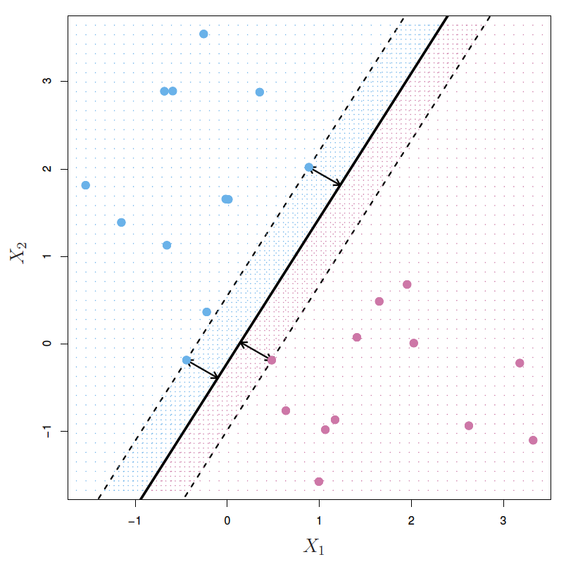
The Non-separable Case:
- The maximal margin classifier is a very natural way to perform classification, if a separating hyperplane exists.
- However, in many cases a separating hyperplane does not exist.
- In these situation, we extend the concept of a separating hyperplane in order to develop a hyperplane that almost separates the classes, using a so-called soft margin.
- This generalization of the maximal margin classifier to the non-separable case is known as the support vector classifier.
Support Vector Classifiers:
- Since a hyperplane doesn't always exist, we might be willing to consider a classifier based on a hyperplane that does not perfectly separate the two classes.
- This would lead to greater robustness to individual observations.
- Better classification of most of the training observations.
- It could be worthwhile to misclassify a few training observations in order to do a better job in classifying the remaining observations.
- A support vector classifier does exactly this.
- A support vector classifier is also called a soft margin classifier.
- C is the tuning parameter we use to determine the number and severity of the misclassifications.
- We can think of C as a budget for the amount that the margin can be violated by the n observations.
- If C = 0, then there is no budget for violations to the margin, which is the same as the maximal margin hyperplane.
- As C increases, we become less tolerant of violations to the margin.
- C controls the bias-variance trade-off.
- Small C leads to low bias and high variance.
- Larger C high bias and low variance.
- The fact that the support vector classifier's decision rule is based on a potentially small subset of the training observations (the support vectors) means that it is quite robust to the behavior of observations that are far away from the hyperplane.
- This is very different from other classifiers.
Support Vector Machines:
- The support vector classifier works when the class boundaries are linear. However, those boundaries are non-linear we must enlarge the feature space to create linear boundaries.
- This is the approach of the support vector machine .
- The support vector machine (SVM) is an extension of the support vector classifier that results from enlarging the feature space using kernels (kernel trick).
- The kernel tick is an efficient computational approach to enlarging our feature space in order to accommodate a non-linear boundary between classes.
SVMs with More than Two Classes:
- The concept of separating hyperplanes upon which SVMs are based does not lend itself naturally to more than two classes.
- Two solutions are the:
- One-Versus-One Classification
- Also called all-airs classification
- Perform
kC2SVM classifications between all classes and assign the test observation to the class to which it is most frequently assigned in the pairwise classification. (round robins)
- One-Versus-All Classification
- Fit the SVM with one class against all of the other classes combined.
- One-Versus-One Classification
Relationship to Logistic Regression:
- SVM and logistic regression often give very similar results.
- When the classes are well separated, SVMs tend to behave better than logistic regression; in more overlapping regimes, logistic regression is often preferred.
- Main goal of support vector machines: try and find a plane that separates the classes in feature space.
- If we cannot do that, we can get creative by:
- Softening what we mean by 'separates'
- Enrich and enlarge the feature space so that separation is possible.
- If we cannot do that, we can get creative by:
- What is a hyperplane?
- A hyperplane in p dimensions is a flat affine subspace of dimension p-1.
- In p=2 dimensions, a hyperplane is a line.
- Maximal Margin Classifier: Among all separating hyperplanes, find the one that makes the biggest gap or margin between the two classes.
- The support vector classifier maximizes a soft margin.
- We have a budget for class overlap when creating the hyperplane.
- C is the regularization parameter to control the budget.
- When no linear separating boundary exists and our soft margin can't help us, we can use the kernel trick with feature expansion to solve the problem.
- Feature expansion involves enlarging the features by including transformations (i.e., X, X^2^, X^3^).
- Hence go from a p-dimensional space to a M > p dimensional space.
- We then fit a support-vector classifier in the enlarged space.
- This results in a non-linear decision boundary in the original space.
- Kernel functions serve this same purpose.
- Examples: Radial Kernel, Polynomial Kernel
- When we have more than two classes we can use a few strategies:
- OVA (One vs. All): Fit K different 2-class SVM classifiers; each class versus the rest. Classify the test observation to the class for which the prediction is largest.
- OVO (One vs. One): Fit all pairwise classifiers. Classify the test observation to the class that wins the most pairwise competitions.
- When should you use Logistic Regression of SVM?
- When classes are (nearly) separable, SVM does better than LR. So does LDA.
- When not, LR (with ridge penalty) and SVM very similar.
- If you wish to estimate probabilities, LR is the choice.
- For nonlinear boundaries, kernel SVMs are popular. Can use kernels with LR and LDA, but computations are more expensive.
- Unsupervised learning: a set of statistical tools intended for the setting in which we have only a set of features without any associated response variable.
- We are not interested in prediction, instead we are looking for patterns or groupings in the observations.
- Two most common unsupervised methods:
- PCA
- clustering
The Challenge of Unsupervised Learning:
- Unsupervised learning is often more challenging than supervised learning. It's more subjective, and there is no simple goal for the analysis, such as prediction of a response.
- Unsupervised learning is often performed as part of an exploratory data analysis.
- It can be hard to assess the results obtained from unsupervised learning methods, since there is no universally accepted mechanism for performing cross validation on an independent data set.
- There is no way to check out work because we don't know the true answer.
Principal Components Analysis:
- When faced with a large set of correlated variables, principal components allow us to summarize this set with a smaller number of representative variables that collectively explain most of the variability in the original set.
- Principal component analysis (PCA) refers to the process by which principal components are computed, and the subsequent use of these components in understanding the data.
- PCA is an unsupervised approach since it involves only a set of features.
What are Principal Components?:
- PCA is a tool to find a low-dimensional representation of a data set that contains as much as possible of the variation.
- The idea is that each of the n observations lives in p-dimensional space, but not all of these dimensions are equally interesting. PCA seeks a small number of dimensions that are as interesting as possible, where the concept of interesting is measured by the amount that the observations vary along each dimension.
- Each of the dimensions found by PCA is a linear combination of the p features.
- The first principal component is the normalized linear combination of the features that has the largest variance.
- The second principal component is the linear combination of the features that has maximal variance out of all linear combinations that are uncorrelated with the first principal component (i.e., orthogonal to the first principal component).
Another Interpretation of Principal Components:
- Principal components provide low-dimensional linear surfaces that are closest to the observations.
- The first principal component loading vector has a very special property: it is the line in p-dimensional space that is closest to the n observations (using average squared Euclidian distance as a measure of closeness).
- The appeal of this interpretation is clear: we seek a single dimension of the data that lies as close as possible to all of the data points, since such a line will likely provide a good summary of the data.
- The first principal component loading vector has a very special property: it is the line in p-dimensional space that is closest to the n observations (using average squared Euclidian distance as a measure of closeness).
Scaling the Variables:
- Before PCA is performed, the variables should be centered to have mean zero.
- The one exception being that if the features are originally measured in the same units then there is no need to scale them.
- The results obtained when we perform PCA will depend on whether the variables have been individually scaled.
Deciding How Many Principal Components to Use:
- In general, a n x p data matrix X has min(n - 1, p) distinct principal components.
- However, we usually are not interested in all of them.
- We typically decide on the number of principal components required to visualize the data by examining a scree plot.
- Scree plot is also known as an elbow plot.
- This is done by eyeballing the scree plot, and looking for a point at which the proportion of variance explained by each subsequent principal component drops off (i.e., the elbow).
Clustering Methods:
- Clustering refers to a very broad set of techniques for finding subgroups, or clusters, in a data set.
- We seek to partition observations in distinct groups so that the observations within each group are quite similar to each other, while observations in different groups are quite different from each other.
- Both clustering and PCA seek to simplify the data via a small number of summaries, but their mechanisms are different:
- PCA looks to find a low-dimensional representation of the observations that explain a good fraction of the variance.
- Clustering looks to find homogeneous subgroups among the observations
- Two most common types of clustering:
- K-means clustering
- We seek to partition the observations into a pre-specified number of clusters.
- hierarchical clustering
- We do not know in advance how many clusters we want; we instead end up with a tree-like representation of the observations, called a dendogram, that allows us to view at once the clusterings obtained for each possible number of clusters, from 1 to n.
- K-means clustering
K-Means Clustering:
- K-Means clustering is an approach for partitioning a data set into K distinct, non-overlapping clusters.
- To perform K-means clustering, we must first specify the desired number of clusters K; then the k-means algorithm will assign each observation to exactly one of the K clusters.
- The idea behind K-means clustering is that a good clustering is one for which the within-cluster variation is as small as possible.
- The within-cluster variation is a measure of the amount by which the observations within a cluster differ from each other.
- The most common way to measure within-group variation is squared euclidean distance.
- The K-means algorithm finds a local rather than a global optimum so the results depend on how the clusters are initialized.
- For this reason, it is important to run the algorithm multiple times from different random initial configurations.
- For this reason, it is important to run the algorithm multiple times from different random initial configurations.

Hierarchical Clustering:
- One potential disadvantage of K-means clustering is that it requires us to pre-specify the number of clusters in K.
- Hierarchical clustering is an alternative approach which does not require that we commit to a particular choice of K.
- There are two types of hierarchical clustering:
- bottom-up
- agglomerative
- The four most common types of linkage are:
- complete
- average
- single
- centroid
- Euclidean distance is commonly used as the dissimilarity measure between clusters.
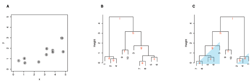
- Unsupervised learning involves situations in which we only observe features without out an associated target.
- We are not interested in prediction, but only pattern recognition.
- The goal of unsupervised learning is to discover interesting things about the measurements: Can we discover subgroups among the variables or among the observations.
- Two key methods of unsupervised learning:
- Principal Components Analysis (PCA): A tool used for data visualization or data pre-processing before supervised techniques are applied
- PCA produces a low-dimensional representation of a dataset. It finds a sequence of linear combinations of the variables that have maximal variance, and are mutually uncorrelated.
- Apart from producing derived variables for use in supervised learning problems, PCA also serves as a tool for data visualization.
- Clustering: a broad class of methods for discovering unknown subgroups in data.
- Principal Components Analysis (PCA): A tool used for data visualization or data pre-processing before supervised techniques are applied
- Unsupervised learning is more subjective than supervised learning, as there is no simple goal for the analysis, such as prediction of a response.
- However, unsupervised learning techniques are growing in importance in a number of fields.
- However, there is an advantage of unsupervised learning in that it is often easier to obtain unlabeled data.
- Features must be scaled before performing PCA.
- If we use principal components as a summary of our data, how many components are sufficient?
- No simple answer to this question, as cross-validation is not available for this purpose.
- However, we could use cross validation within a regression to decide how many principal components to use.
- Use of scree plot; look for the elbow.
- Clustering refers to a very broad set of techniques for finding subgroups, or clusters in a data set.
- We seek a partition of the data into distinct groups so that the observations within each group are quite similar to each other.
- To make this concrete, we must define what it means for two or more observations to be similar or different.
- This is often a domain-specific consideration that must be made based on knowledge of the data being studied.
- PCA vs. Clustering:
- PCA looks for a low-dimensional representation of the observations that explains a good fraction of the variance.
- Clustering looks for homogeneous subgroups among the observations.
- Two most common clustering methods:
- k-Means Clustering
- We seek to partition the observations into pre-specified number of clusters.
- The idea being k-Means clustering is that a good clustering is one for which the within-cluster variation is as small as possible.
- We want to partition the observations in K clusters such that the total within-cluster variation, summed over all K clusters, is as small as possible.
- We typically use euclidean distance to define within-cluster variation.
- Not guaranteed to give global minimum.
- Hierarchical Clustering:
- We do not know in advance how many clusters we want; in fact, we end up with a tree-like visual representation of the observations, called a dendogram, that allows us to view at once the clusterings obtained from each possible number of clusters, from 1 to n.
- k-Means Clustering
- K-Means clustering requires us to pre-specify the number of clusters K. This can be a disadvantage.
- Hierarchical clustering is an alternative approach which does not require that we commit to a particular choice of K.
- The most common hierarchical clustering is called bottom-up or agglomerative clustering, which refers to the fact that a dendogram is built starting from the leaves and combining clusters up to the trunk.